audpc

library(epifitter)     # Para AUDPC(), cv.model(), e o dataset PowderyMildew
library(ggplot2)       # Para visualizações com ggplot
library(dplyr)         # Para filter(), group_by(), summarise(), pipe (%>%) ou |>
library(DHARMa)        # Para simulate_residuals()
library(emmeans)       # Para emmeans() e cld()
library(multcomp)

AUDPC

Esse script em R realiza uma análise da severidade de oídio (um tipo de doença fúngica) em diferentes sistemas de irrigação e níveis de umidade, usando gráficos, cálculo da área abaixo da curva de progresso da doença (AUDPC), ANOVA e comparação de médias. Abaixo está a interpretação detalhada e explicativa de cada etapa e da tabela final:

library(epifitter)

oidio <- PowderyMildew
#Vários tipos de gráficos


oidio |>
  ggplot(aes(factor (time), sev)) +
  geom_jitter(width=0.1) +
  facet_wrap(irrigation_type ~ moisture)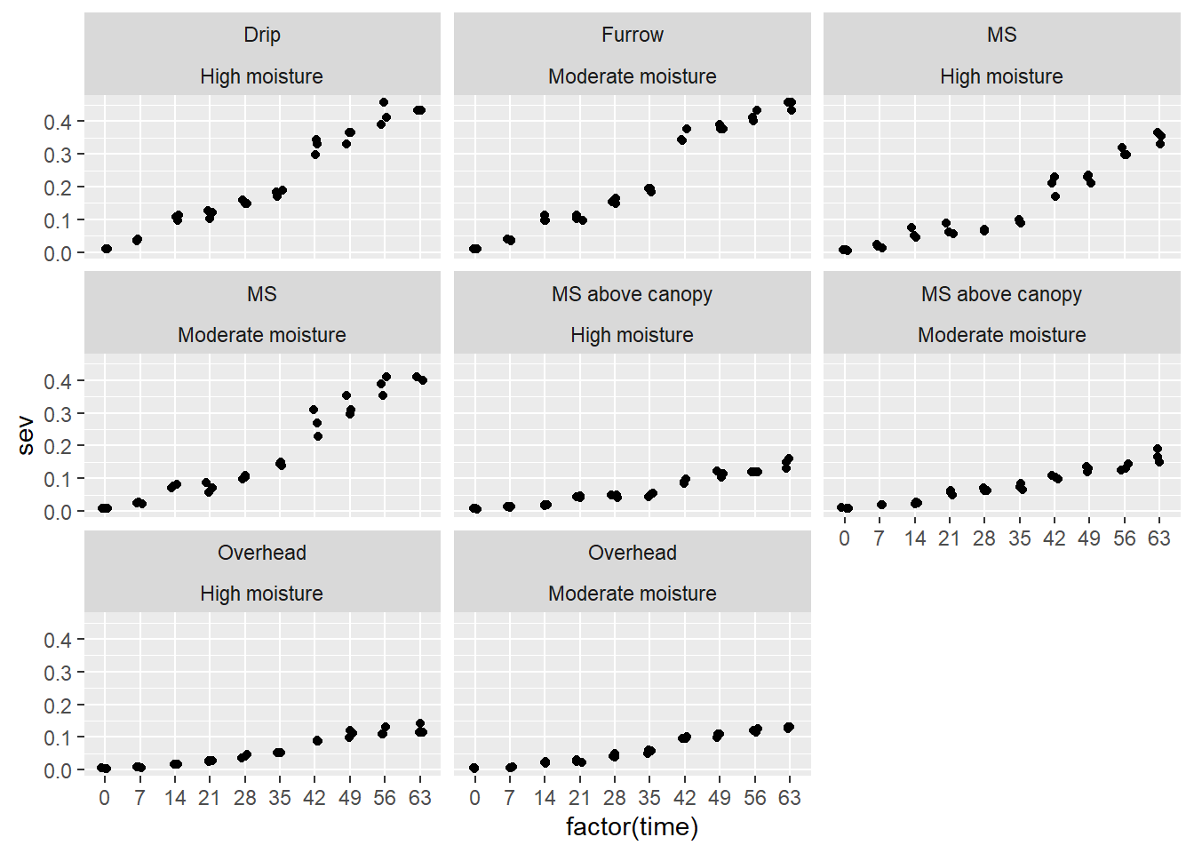

oidio |>
  ggplot(aes(factor (time), sev)) +
  geom_jitter(width=0.1) +
  facet_grid(moisture ~ irrigation_type)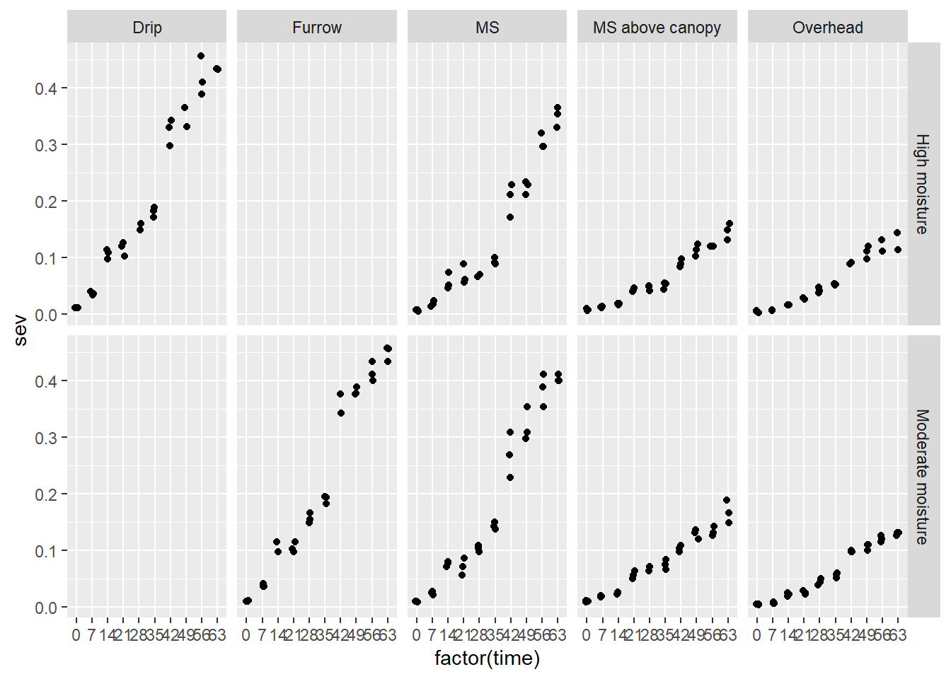

oidio2 <- oidio|>
  filter(irrigation_type %in% c("MS", "MS above canopy", "Overhead")) 
oidio2 |> ggplot(aes(time, sev)) +
  geom_point() +
  facet_grid(moisture ~ irrigation_type)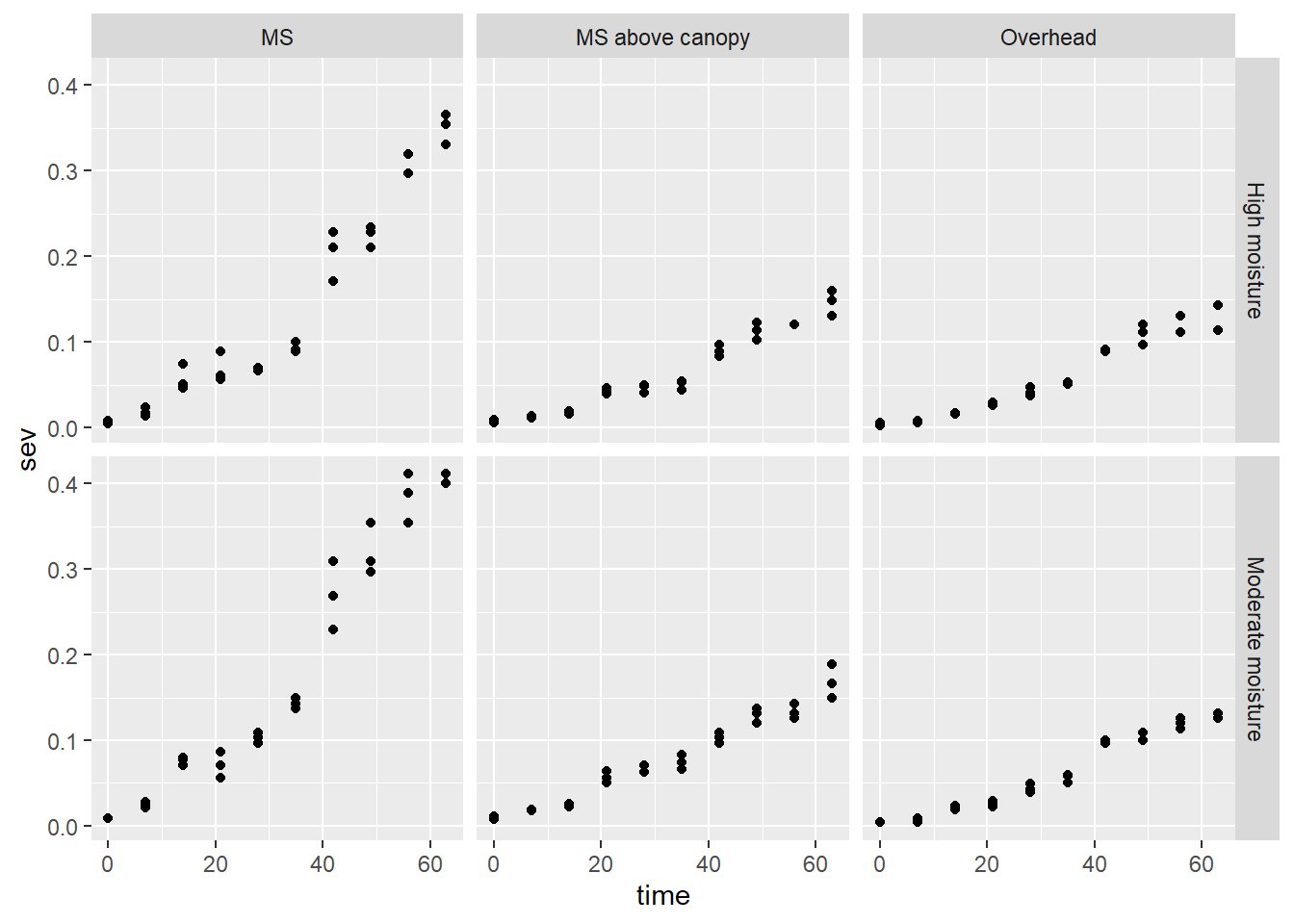

#Calcular média abaixo da curva

oidio3 <- oidio2 |> 
  group_by(irrigation_type, moisture, block) |> 
  summarise(AUDPC = AUDPC(time, sev))

#Plotar área abaixo da curva

oidio3 |> 
  ggplot(aes(irrigation_type, AUDPC, color = moisture)) +
  geom_point(size = 2) + 
  scale_y_continuous(limits = c(0,20))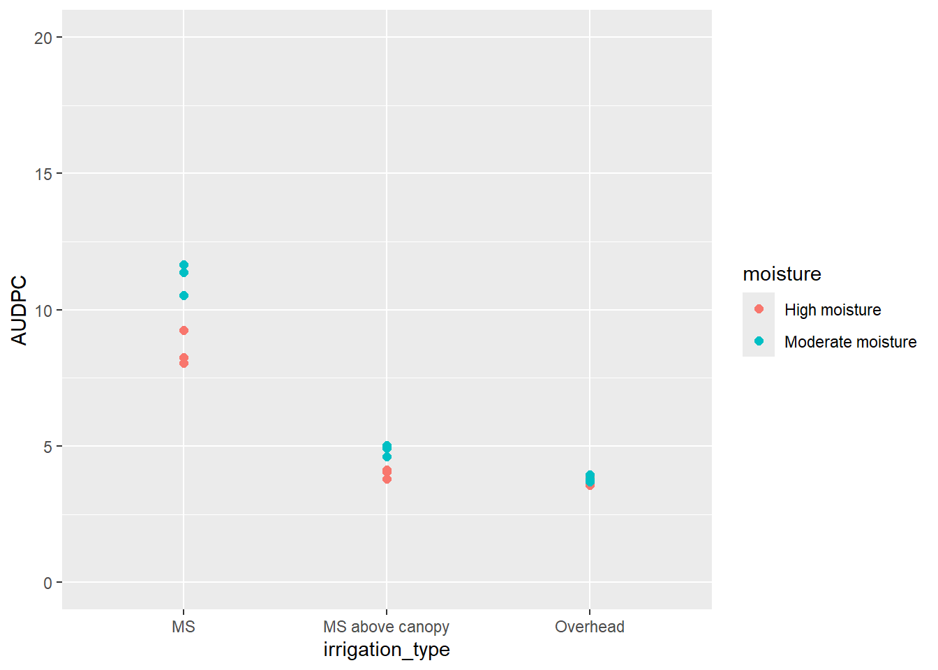

#Verificar se há diverenças
#Fazer ANOVA

oidio4 <- lm(AUDPC ~ irrigation_type*moisture, data = oidio3)
anova(oidio4)

Analysis of Variance Table

Response: AUDPC
                         Df  Sum Sq Mean Sq F value    Pr(>F)    
irrigation_type           2 134.341  67.170 451.721 5.073e-12 ***
moisture                  1   6.680   6.680  44.924 2.188e-05 ***
irrigation_type:moisture  2   5.104   2.552  17.162 0.0003022 ***
Residuals                12   1.784   0.149                      
---
Signif. codes:  0 '***' 0.001 '**' 0.01 '*' 0.05 '.' 0.1 ' ' 1

plot(simulateResiduals(oidio4))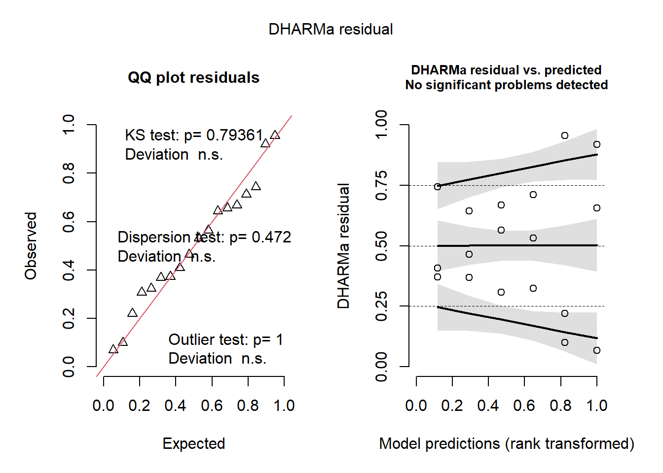

#Ver visualmente se é diferente
medias_oidio <- emmeans(oidio4, ~ moisture | irrigation_type)
cld(medias_oidio)

irrigation_type = MS:
 moisture          emmean    SE df lower.CL upper.CL .group
 High moisture       8.52 0.223 12     8.04     9.01  1    
 Moderate moisture  11.18 0.223 12    10.70    11.67   2   

irrigation_type = MS above canopy:
 moisture          emmean    SE df lower.CL upper.CL .group
 High moisture       3.99 0.223 12     3.51     4.48  1    
 Moderate moisture   4.86 0.223 12     4.37     5.34   2   

irrigation_type = Overhead:
 moisture          emmean    SE df lower.CL upper.CL .group
 High moisture       3.68 0.223 12     3.20     4.17  1    
 Moderate moisture   3.81 0.223 12     3.33     4.30  1    

Confidence level used: 0.95 
significance level used: alpha = 0.05 
NOTE: If two or more means share the same grouping symbol,
      then we cannot show them to be different.
      But we also did not show them to be the same.

medias_oidio2 <- emmeans(oidio4, ~ irrigation_type | moisture)
cld(medias_oidio2)

moisture = High moisture:
 irrigation_type emmean    SE df lower.CL upper.CL .group
 Overhead          3.68 0.223 12     3.20     4.17  1    
 MS above canopy   3.99 0.223 12     3.51     4.48  1    
 MS                8.52 0.223 12     8.04     9.01   2   

moisture = Moderate moisture:
 irrigation_type emmean    SE df lower.CL upper.CL .group
 Overhead          3.81 0.223 12     3.33     4.30  1    
 MS above canopy   4.86 0.223 12     4.37     5.34   2   
 MS               11.18 0.223 12    10.70    11.67    3  

Confidence level used: 0.95 
P value adjustment: tukey method for comparing a family of 3 estimates 
significance level used: alpha = 0.05 
NOTE: If two or more means share the same grouping symbol,
      then we cannot show them to be different.
      But we also did not show them to be the same.

residuosoidio4 <- residuals(oidio4)
sd_res <- sd(residuosoidio4)
media_fitted <- mean(fitted(oidio4))
cv <- (sd_res / media_fitted) * 100
print(cv)

[1] 5.392371

	H moisture	M moisture
Irrigation
MS	8,52 Aa	11,18 Ab
MS AC	3,99 Ba	4,86 Bb
Overhead	3,68 Ba	3,81 Ca
CV = 5,39